
Introduction to finite rotations in BeamMe#
When working with Cosserat continua in 3D, the mathematical treatment of finite rotations is required. This example gives an overview of the finite rotation functionality in BeamMe. For a more comprehensive and theoretical overview of finite rotations, the interested reader is referred to:
Crisfield, M. A., 1997, Non-Linear Finite Element Analysis of Solids and Structures, Volume 2, Advanced Topics, Wiley & Sons.
Krenk, S., 2009, Non-Linear Modeling and Analysis of Solids and Structures, Cambridge University Press.
All finite rotation functionality within BeamMe can be accessed via the Rotation class. Each instance of this class represents an element of the special orthogonal group \(\SO\).
The rotation class can be imported with
[1]:
from beamme.core.rotation import Rotation
Different finite rotation representations#
Internally, BeamMe uses a unit-quaternion representation to store the \(\SO\) element which provides an efficient and singularity free representation. However, the user can input and output all major representations of large rotations via the Rotation class. Supported representations are:
Rotation axis and angle: From an user input point of view, this is the most natural way to create a large rotation object. This is the default initialization method via the constructor, i.e.,
rotation = Rotation(axis, angle)Rotation (pseudo-) vector: can be done with
rotation = Rotation.from_rotation_vector(psi)Unit-quaternion: can be done with
rotation = Rotation.from_quaternion(q)Rotation matrix: can be done with
rotation = Rotation.from_rotation_matrix(R)
Lets start with the creation of a unit rotation from all different representations
[2]:
# Unit rotation from the axis/angle constructor.
# Note: In this case the rotation axis does not matter, but it can not be a 0 vector
unit_rotation_from_axis_angle = Rotation([1, 1, 1], 0.0)

# Unit rotation from a rotation vector
unit_rotation_from_rotation_vector = Rotation.from_rotation_vector([0, 0, 0])

# Unit rotation from a quaternion
unit_rotation_from_quaternion = Rotation.from_quaternion([1, 0, 0, 0])

# Unit rotation from a rotation matrix (in this case the identity matrix)
unit_rotation_from_rotation_matrix = Rotation.from_rotation_matrix(
    [[1, 0, 0], [0, 1, 0], [0, 0, 1]]
)

# An empty constructor also creates a unit rotation
unit_rotation_constructor = Rotation()
We can now check that all created rotations are equal
[3]:
assert unit_rotation_constructor == unit_rotation_from_axis_angle
assert unit_rotation_constructor == unit_rotation_from_rotation_vector
assert unit_rotation_constructor == unit_rotation_from_quaternion
assert unit_rotation_constructor == unit_rotation_from_rotation_matrix
In the next step, lets create rotations around the \(x\)-axis with an angle of \(\pi/3\).
Note: The rotation matrix representing this rotation is
[4]:
import numpy as np

# Rotation from the axis/angle constructor
# We define the x-axis as rotation axis and the angle as the second argument
rotation_from_axis_angle = Rotation([1, 0, 0], np.pi / 3)

# Rotation from a rotation vector
rotation_from_rotation_vector = Rotation.from_rotation_vector([np.pi / 3, 0, 0])

# Rotation from a rotation matrix
rotation_from_rotation_matrix = Rotation.from_rotation_matrix(
    np.array(
        [
            [1, 0, 0],
            [0, np.cos(np.pi / 3), -np.sin(np.pi / 3)],
            [0, np.sin(np.pi / 3), np.cos(np.pi / 3)],
        ]
    )
)
Again, we can check that all initializations result in the same rotation object
[5]:
assert rotation_from_axis_angle == rotation_from_rotation_vector
assert rotation_from_axis_angle == rotation_from_rotation_matrix
We can also extract the different finite rotation parameterizations from any Rotation object
Note: The axis/angle representation is not unique and mainly useful as an input, therefore, no get_axis_angle method exists.
[6]:
rotation = Rotation([1, 0, 0], np.pi / 3)

print(f"Quaternion representation:\n{rotation.get_quaternion()}\n")
print(f"Rotation vector representation:\n{rotation.get_rotation_vector()}\n")
print(f"Rotation matrix representation:\n{rotation.get_rotation_matrix()}")
Quaternion representation:
[0.8660254 0.5       0.        0.       ]

Rotation vector representation:
[1.04719755 0.         0.        ]

Rotation matrix representation:
[[ 1.         0.         0.       ]
 [ 0.         0.5       -0.8660254]
 [ 0.         0.8660254  0.5      ]]
Finite rotation calculations#
For mesh creation purposes it is essential to compose multiple rotations, calculate relative rotations or rotate a vector by a given rotation. With the Rotation class this can easily be achieved in a pythonic way.
Rotation composition#
Lets start of with the rotation \(\triad_{x}\) (around \(x\)-axis with angle \(\pi/2\)) and \(\triad_{y}\) (around \(y\)-axis with angle \(\pi/2\))
[7]:
lambda_x = Rotation([1, 0, 0], 0.5 * np.pi)
lambda_y = Rotation([0, 1, 0], 0.5 * np.pi)
We can visualize these rotations
[8]:
import vtk  # We need to import vtk before pyvista for the TeX labels to work # noqa: F401, I001
import pyvista as pv

pv.set_jupyter_backend("trame")


# Utility functionality for this example
from example_1_finite_rotations_utils import (
    PyVistaPlotter,
    add_cube_plot,
    print_matrix,
    print_rotation_matrix,
)

with PyVistaPlotter(shape=(1, 3), window_size=(1400, 500)) as plotter:
    add_cube_plot(plotter, 0, 0, Rotation(), "Original object")
    add_cube_plot(
        plotter,
        0,
        1,
        lambda_x,
        "Rotated around the $x$-axis\nwith the angle $\\pi/2$ ($\\Lambda_{x}$)",
    )
    add_cube_plot(
        plotter,
        0,
        2,
        lambda_y,
        "Rotated around the $y$-axis\nwith the angle $\\pi/2$ ($\\Lambda_{y}$)",
    )
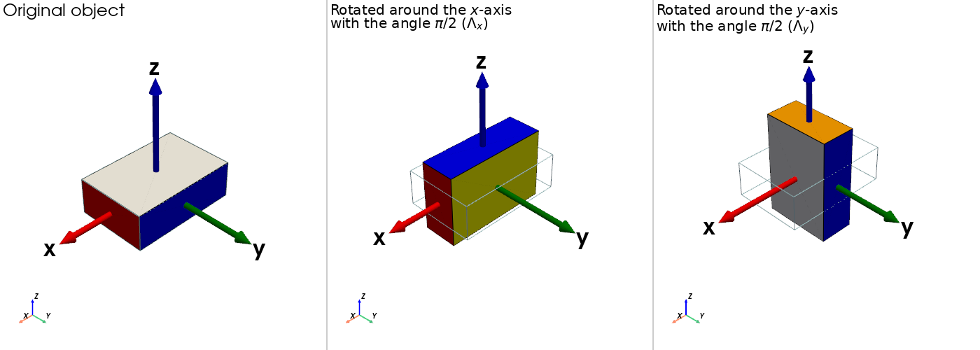
We can now compute the composition of the two rotations \(\triad_{yx}\), i.e., first applying \(\triad_{x}\) then \(\triad_{y}\). This can be done with the standard multiply operator *:
[9]:
lambda_yx = lambda_y * lambda_x
print_rotation_matrix("lambda_yx", lambda_yx)
lambda_yx:
[[ 0.  1.  0.]
 [ 0.  0. -1.]
 [-1.  0.  0.]]
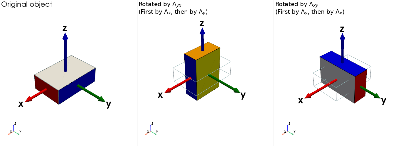
An important property for elements of \(\SO\) is, that multiplications are non-commutative, i.e., the order of the elements in the multiplication matters. Thus, \(\triad_{yx} = \triad_{y} \triad_{x} \ne \triad_{x} \triad_{y} = \triad_{xy}\). We can easily check this
[10]:
lambda_xy = lambda_x * lambda_y
print_rotation_matrix("lambda_xy", lambda_xy)

if lambda_xy == lambda_yx:
    print("Rotations lambda_yx and lambda_xy are equal!")
else:
    print("Rotations lambda_yx and lambda_xy are NOT equal!")

assert not lambda_yx == lambda_xy
lambda_xy:
[[ 0.  0.  1.]
 [ 1.  0. -0.]
 [-0.  1.  0.]]
Rotations lambda_yx and lambda_xy are NOT equal!
We can also visualize that these rotations are not equal to each other
[11]:
with PyVistaPlotter(shape=(1, 3), window_size=(1400, 500)) as plotter:
    add_cube_plot(plotter, 0, 0, Rotation(), "Original object")
    add_cube_plot(
        plotter,
        0,
        1,
        lambda_yx,
        "Rotated by $\\Lambda_{yx}$\n(First by $\\Lambda_x$, then by $\\Lambda_y$)",
    )
    add_cube_plot(
        plotter,
        0,
        2,
        lambda_xy,
        "Rotated by $\\Lambda_{xy}$\n(First by $\\Lambda_y$, then by $\\Lambda_x$)",
    )
Rotation inversion#
Rotations can also be inverted. This allows to easily calculate \(\triad_{y}\) from \(\triad_{yx}\) and \(\triad_{x}\) via \(\triad_{y} = \triad_{yx} (\triad_{x})^{-1}\)
[12]:
lambda_y_computed = lambda_yx * lambda_x.inv()
assert lambda_y == lambda_y_computed
Rotating a vector#
In many cases, we need to compute the rotation of a vector \(\vv{a} \in \R{3}\). For example \(\vv{a}' = \triad_{21} \vv{a}\). This can be done by simply using the * operator between a Rotation object and a 3D vector:
[13]:
r = [1, 2, 3]
r_prime = lambda_yx * r
print(f"Rotated vector: {r_prime}")
Rotated vector: [ 2. -3. -1.]
Alternatively, we can also use the rotation matrix representation to rotate a vector:
[14]:
rotation_matrix = lambda_yx.get_rotation_matrix()
r_prime_matrix = rotation_matrix @ np.array(r)
print(f"Rotated vector (via rotation matrix): {r_prime_matrix}")
Rotated vector (via rotation matrix): [ 2. -3. -1.]
Advanced features#
BeamMe also provides advanced finite rotation functionality such as smallest rotation mappings and transformation matrices between additive and multiplicative increments.
Smallest rotation mapping#
A smallest rotation mapping calculates the triad \(\triad_{sr}\) that results from the smallest rotation (rotation without twist) from the triad \(\triad\) such that the rotated first basis vector aligns with \(\vv{t}\). In mathematical terms, \(\vv{t} = \triad_{sr} \vv{e}_1\), where the rotation vector for the relative triad \(\triad_{rel} = \triad_{sr}(\triad)^{-1}\) is a minimum.
[15]:
from beamme.core.rotation import smallest_rotation

rotation = Rotation([1, 2, 3], np.pi / 6.0)
lambda_sr = smallest_rotation(rotation, [1, 0.5, 0])
print(f"First basis vector of lambda_sr: {lambda_sr * [1, 0, 0]}")
First basis vector of lambda_sr: [ 8.94427191e-01 4.47213595e-01 -6.93889390e-18]
Transformation matrix \(\mm{T}\)#
The infinitesimal variations of the rotation tensor \(\triad(\vv{\psi})\) (where \(\vv{\psi}\) is the rotation vector) can be expressed in two ways:
Additive Variation:
\[\delta \triad = \frac{d}{d\epsilon} \bigg|_{\epsilon=0} \triad(\vv{\psi} + \epsilon \delta \vv{\psi}) = \frac{\partial \triad(\vv{\psi})}{\partial \vv{\psi}} \delta \vv{\psi}\]This represents the standard definition of partial differentiation, which is based on additive increments.
Multiplicative Variation (also referred to as the spin vector variation):
\[\delta \triad = \frac{d}{d\epsilon} \bigg|_{\epsilon=0} \triad(\epsilon \delta \vv{\theta}) \triad(\vv{\psi}) = \mm{S}(\delta \vv{\theta}) \triad(\vv{\psi})\]Here, \(\mm{S}(\delta \vv{\theta})\) is the skew-symmetric matrix corresponding to the axial vector \(\delta \vv{\theta}\).
The two variations are related through the transformation matrix \(\mm{T}(\vv{\psi})\), which satisfies:
BeamMe provides an explicit implementation of \(\mm{T}\) and \(\mm{T}^{-1}\) via the Rotation class:
[16]:
rotation = Rotation([1, 2, 3], np.pi / 6.0)
print_matrix("Transformation matrix", rotation.get_transformation_matrix())
print_matrix("Transformation matrix inverse", rotation.get_transformation_matrix_inv())
Transformation matrix:
[[ 0.978688    0.21318526 -0.13501951]
 [-0.20662772  0.98360615  0.07980514]
 [ 0.14485581 -0.06013252  0.99180308]]
Transformation matrix inverse:
[[ 0.95814897 -0.19871589  0.1464276 ]
 [ 0.21159313  0.9678069  -0.04906898]
 [-0.12711174  0.0877007   0.98390345]]